Working with Data¶

Describing Data using Pandas¶

In this first section, we will use the Pandas package to explore and describe data from O’Connell, K., Berluti, K., Rhoads, S. A., & Marsh, A. A. (2021). Reduced social distancing during the COVID-19 pandemic is associated with antisocial behaviors in an online United States sample. PLoS ONE.

This study assessed whether social distancing behaviors (early in the COVID-19 pandemic) was associated with self-reported antisocial behavior.

# Remember: Python requires you to explictly "import" libraries before their functions are available to use. We will always specify our imports at the beginning of each notebook.
import pandas as pd, numpy as np

Here, we will load a dataset as a pandas.DataFrame, and investigate its attributes. We will see N rows for each subject, and M columns for each variable.

Loading data¶

# here, we are just going to download data from the web
url = 'https://raw.githubusercontent.com/shawnrhoads/gu-psyc-347/master/docs/static/data/OConnell_COVID_MTurk_noPII_post_peerreview.csv'

# load data specified in `filename` into dataframe `df`
df = pd.read_csv(url)

# check type of df
type(df)

pandas.core.frame.DataFrame

# how many rows and columns are in df?
print(df.values.shape) # N x M

(131, 126)

Looks like we will have 131 rows (usually subjects, but can be multiple observations per subject) and 126 columns (usually variables)

# let's output the first 5 rows of the df
print(df.head())

   subID  mturk_randID  suspect_itaysisso        Country Region  \
 1001          8797                  0  United States     CT   
 1002          3756                  0  United States     IL   
 1003          3798                  0  United States     OH   
 1004          2965                  0  United States     TX   
 1005          5953                  0  United States     NC   

                                        ISP loc_US       loc_state  \
AS7015 Comcast Cable Communications, LLC    Yes     Connecticut   
              AS7018 AT&T Services, Inc.    Yes      California   
      AS10796 Charter Communications Inc    Yes            Ohio   
              AS7018 AT&T Services, Inc.    Yes           Texas   
          AS20115 Charter Communications    Yes  North Carolina   

   loc_zipcode          loc_County  ...  education_4yr  STAB_total_centered  \
       6511    New Haven County  ...              0            -3.946565   
      90280  Los Angeles County  ...              0            39.053436   
      44883       Seneca County  ...              0            40.053436   
      77019       Harris County  ...              1            -9.946565   
      28334      Sampson County  ...              0           -17.946566   

   STAB_total_min32  silhouette_dist_X_min81 silhouette_dist_X_inches  \
              19                    441.0               110.332750   
              62                    287.0                71.803856   
              63                    313.0                78.308731   
              13                    452.0               113.084820   
               5                    297.0                74.305733   

  violated_distancing STAB_rulebreak_rmECONOMIC  STAB_total_rmECONOMIC  \
                 0                         9                     48   
                 1                        24                     88   
                 0                        23                     85   
                 0                         8                     42   
                 0                         8                     34   

   STAB_total_rmECONOMIC_centered  household_income_coded_centered  
                     -2.076336                         1.269231  
                     37.923664                        -3.730769  
                     34.923664                        -2.730769  
                     -8.076336                              NaN  
                    -16.076336                        -2.730769  

[5 rows x 126 columns]

Creating custom DataFrames¶

We can also create our own dataframe. For example, here’s a dataframe containing 20 rows and 3 columns of random numbers.

sim_df = pd.DataFrame(np.random.randn(20, 3), index=range(0,20), columns=["column A", "column B", "column C"])
print(sim_df)

    column A  column B  column C
 0.392950 -1.180451 -0.838785
-0.389347  1.017663 -0.424514
 1.856004  0.285378 -0.120892
-0.659527  1.241937  0.754542
-2.169041  0.080437 -0.336512
 1.889987  1.048956  0.740878
 0.589985  0.581513  0.167113
 1.844384 -0.015155 -0.285773
-1.958567 -0.898125 -0.974897
 0.005468 -0.030749 -0.672078
-0.850622 -1.058297 -0.411733
-0.400981 -0.988033 -1.489113
1.623723  0.496788 -1.979738
1.364699  0.467905  0.228723
-0.569220  0.175305  1.545127
0.559054  0.083730 -1.018083
-0.800119 -0.580347  1.251444
0.797440 -0.415382  0.120163
-2.143062  0.005168 -0.432682
-1.527358  0.585114 -1.219528

We can change the column names using list comprehension

# e.g., change to upper case
sim_df.columns = [x.upper() for x in sim_df.columns]
print(sim_df.head()) #display first 5 rows

   COLUMN A  COLUMN B  COLUMN C
0.392950 -1.180451 -0.838785
-0.389347  1.017663 -0.424514
1.856004  0.285378 -0.120892
-0.659527  1.241937  0.754542
-2.169041  0.080437 -0.336512

# e.g., change to last element in string
sim_df.columns = [x[-1] for x in sim_df.columns]
print(sim_df.tail()) #display last 5 rows

           A         B         C
0.559054  0.083730 -1.018083
-0.800119 -0.580347  1.251444
0.797440 -0.415382  0.120163
-2.143062  0.005168 -0.432682
-1.527358  0.585114 -1.219528

Concatenating DataFrames¶

We can concatenate multiple dataframes containing the same columns (e.g., [‘A’,’B’,’C’]) using pd.concat(). This will stack rows across dataframes.

Usage:

pd.concat(
    objs,
    axis=0,
    join="outer",
    ignore_index=False,
    keys=None,
    levels=None,
    names=None,
    verify_integrity=False,
    copy=True,
)

np.zeros((3,3))

array([[0., 0., 0.],
       [0., 0., 0.],
       [0., 0., 0.]])

# create two new dataframes 

# the first will contain only zeros 
sim_df1 = pd.DataFrame(np.zeros((3, 3)), index=[20,21,22], columns=["A", "B", "C"])

# the second will contain only ones
sim_df2 = pd.DataFrame(np.ones((3, 3)), index=[23,24,25], columns=["A", "B", "C"])

sim_dfs = [sim_df, sim_df1, sim_df2] # as list of dfs
result = pd.concat(sim_dfs)
print(result)

           A         B         C
 0.392950 -1.180451 -0.838785
-0.389347  1.017663 -0.424514
 1.856004  0.285378 -0.120892
-0.659527  1.241937  0.754542
-2.169041  0.080437 -0.336512
 1.889987  1.048956  0.740878
 0.589985  0.581513  0.167113
 1.844384 -0.015155 -0.285773
-1.958567 -0.898125 -0.974897
 0.005468 -0.030749 -0.672078
-0.850622 -1.058297 -0.411733
-0.400981 -0.988033 -1.489113
1.623723  0.496788 -1.979738
1.364699  0.467905  0.228723
-0.569220  0.175305  1.545127
0.559054  0.083730 -1.018083
-0.800119 -0.580347  1.251444
0.797440 -0.415382  0.120163
-2.143062  0.005168 -0.432682
-1.527358  0.585114 -1.219528
0.000000  0.000000  0.000000
0.000000  0.000000  0.000000
0.000000  0.000000  0.000000
1.000000  1.000000  1.000000
1.000000  1.000000  1.000000
1.000000  1.000000  1.000000

We can also concatenate using the rows (setting axis=1)

# the first will contain only zeros 
sim_df3 = pd.DataFrame(np.zeros((3, 3)), index=[1,2,3], columns=["A", "B", "C"])

# the second will contain only ones
sim_df4 = pd.DataFrame(np.ones((3, 3)), index=[2,4,5], columns=["D", "E", "F"])

result2 = pd.concat([sim_df3, sim_df4], axis=1)
print(result2)

     A    B    C    D    E    F
0.0  0.0  0.0  NaN  NaN  NaN
0.0  0.0  0.0  1.0  1.0  1.0
0.0  0.0  0.0  NaN  NaN  NaN
NaN  NaN  NaN  1.0  1.0  1.0
NaN  NaN  NaN  1.0  1.0  1.0

Notice that we have NaNs (not a number) in cells where there were no data (for example, no data in column D for index 1)

We have to be careful because all elements will not merge across rows and columns by default. For example, if the second df also had a column “C”, we will have two “C” columns by default.

# the first will contain only zeros 
sim_df5 = pd.DataFrame(np.zeros((3, 3)), index=[1,2,3], columns=["A", "B", "C"])

# the second will contain only ones
sim_df6 = pd.DataFrame(np.ones((3, 4)), index=[2,4,5], columns=["C", "D", "E", "F"])

result3a = pd.concat([sim_df5, sim_df6], axis=1)
print(result3a)

     A    B    C    C    D    E    F
0.0  0.0  0.0  NaN  NaN  NaN  NaN
0.0  0.0  0.0  1.0  1.0  1.0  1.0
0.0  0.0  0.0  NaN  NaN  NaN  NaN
NaN  NaN  NaN  1.0  1.0  1.0  1.0
NaN  NaN  NaN  1.0  1.0  1.0  1.0

By default, this method takes the “union” of dataframes. This is useful because it means no information will be lost!

But, now we have two columns named “C”. To fix this, we can have pandas rename columns with matching names using the DataFrame.merge() method.

result3b = sim_df5.merge(sim_df6, how='outer', left_index=True, right_index=True)
print(result3b)

     A    B  C_x  C_y    D    E    F
0.0  0.0  0.0  NaN  NaN  NaN  NaN
0.0  0.0  0.0  1.0  1.0  1.0  1.0
0.0  0.0  0.0  NaN  NaN  NaN  NaN
NaN  NaN  NaN  1.0  1.0  1.0  1.0
NaN  NaN  NaN  1.0  1.0  1.0  1.0

We could also take the “intersection” across the two dataframes. We can do that by setting join='inner' (Meaning we only keep the rows that are shared between the two). In the previous case, this would be row ‘2’. All columns would be retained.

result3c = pd.concat([sim_df5, sim_df6], axis=1, join='inner')
print(result3c)

     A    B    C    C    D    E    F
2  0.0  0.0  0.0  1.0  1.0  1.0  1.0

Manipulating DataFrames¶

We can also change values within the dataframe using list comprehension.

# first let's view the column "subID"
df['subID']

    1001
    1002
    1003
    1004
    1005
       ... 
  1160
  1161
  1162
  1163
  1164
Name: subID, Length: 131, dtype: int64

# now, let's change these value by adding a prefix 'sub_' and store in a new column called "subID_2"
df['subID_2'] = ['sub_'+str(x) for x in df['subID']]

df['subID_2']

    sub_1001
    sub_1002
    sub_1003
    sub_1004
    sub_1005
         ...   
  sub_1160
  sub_1161
  sub_1162
  sub_1163
  sub_1164
Name: subID_2, Length: 131, dtype: object

We can also grab specific elements in the dataframe by specifying rows and columns

print(df['age'][df['subID']==1001])

0    21
Name: age, dtype: int64

# if you know the index (row name), then you can use the `pd.DataFrame.loc` method
df.loc[0,'age']

Creating new columns is particularly useful for computing new variables from old variables. For example: for each subject, let’s multiply age by STAB_total.

for index,subject in enumerate(df['subID']):
    df.loc[index,'new_col'] = df.loc[index,'age'] * df.loc[index,'STAB_total'] 

We can extract a column of observations to a numpy array

sub_ids = df['subID'].values

print(sub_ids)

[1001 1002 1003 1004 1005 1007 1011 1013 1014 1015 1016 1017 1021 1022
1024 1026 1028 1029 1032 1033 1034 1035 1040 1043 1044 1045 1047
1049 1051 1053 1054 1056 1057 1058 1059 1060 1061 1062 1063 1064
1068 1069 1070 1071 1072 1073 1074 1075 1076 1077 1078 1079 1080
1083 1084 1085 1086 1087 1088 1089 1090 1091 1092 1093 1094 1095
1098 1099 1100 1101 1102 1104 1105 1107 1108 1109 1110 1111 1112
1114 1115 1116 1117 1118 1119 1120 1121 1122 1123 1124 1125 1126
1128 1129 1130 1131 1132 1133 1134 1135 1136 1137 1138 1139 1141
1145 1146 1147 1148 1149 1150 1151 1152 1154 1155 1156 1157 1158
1161 1162 1163 1164]

print(type(sub_ids))

<class 'numpy.ndarray'>

We can also transpose the dataframe

print(df.T.head())

                             0              1              2              3    \
subID                       1001           1002           1003           1004   
mturk_randID                8797           3756           3798           2965   
suspect_itaysisso              0              0              0              0   
Country            United States  United States  United States  United States   
Region                        CT             IL             OH             TX   

                             4              5              6              7    \
subID                       1005           1007           1011           1013   
mturk_randID                5953           8133           2500           7655   
suspect_itaysisso              0              0              0              0   
Country            United States  United States  United States  United States   
Region                        NC             MA             FL             WI   

                             8              9    ...            121  \
subID                       1014           1015  ...           1154   
mturk_randID                4616           2318  ...           1123   
suspect_itaysisso              0              0  ...              0   
Country            United States  United States  ...  United States   
Region                        MD             LA  ...             NC   

                             122            123            124            125  \
subID                       1155           1156           1157           1158   
mturk_randID                2455           7875           6828           3775   
suspect_itaysisso              0              0              0              0   
Country            United States  United States  United States  United States   
Region                        ID             CA             AZ             CO   

                             126            127            128            129  \
subID                       1160           1161           1162           1163   
mturk_randID                1459           7557           6617           5071   
suspect_itaysisso              0              0              0              0   
Country            United States  United States  United States  United States   
Region                        IL             WA             CA             KY   

                             130  
subID                       1164  
mturk_randID                7031  
suspect_itaysisso              0  
Country            United States  
Region                        MO  

[5 rows x 131 columns]

Statistics with DataFrames¶

We can compute all sorts of descriptive statistics on DataFrame columns using the following methods:

count(): Number of non-null observations
sum(): Sum of values
mean(): Mean of values
median(): Median of values
mode(): Mode of values
std(): Standard deviation of values
min(): Minimum value
max(): Maximum value
abs(): Absolute value
prod(): Product of values
cumsum(): Cumulative sum
cumprod(): Cumulative product

Here are some examples:

# mean of a column
df["age"].mean()

36.33587786259542

# mean of multiple columns
df[["age","STAB_total"]].mean()

age           36.335878
STAB_total    54.946565
dtype: float64

# median of a column
df["age"].median()

34.0

# compute a summary of metrics on columns
df[["age", "STAB_total"]].describe()

	age	STAB_total
count	131.000000	131.000000
mean	36.335878	54.946565
std	10.075569	30.095569
min	21.000000	32.000000
25%	29.500000	35.000000
50%	34.000000	42.000000
75%	41.000000	55.500000
max	65.000000	139.000000

# group means by sex
df.groupby("sex")[["age", "STAB_total"]].mean()

	age	STAB_total
sex
Female	38.264151	49.792453
Male	35.025641	58.448718

# group means by sex and education
df.groupby(["sex","education_coded"])[["age", "STAB_total"]].mean()

		age	STAB_total
sex	education_coded
Female	Four-year college degree (B.A., B.S.)	37.592593	54.074074
	High school graduate or G.E.D.	42.400000	37.600000
	Master's degree (for example, M.B.A., M.A., M.S.)	38.200000	55.800000
	Some college	38.875000	48.875000
	Two-year college degree (A.A., A.S.)	37.375000	40.125000
Male	Doctoral or professional degree (for example, Ph.D., M.D., J.D., D.V.M., D.D.M)	31.500000	34.500000
	Four-year college degree (B.A., B.S.)	35.125000	64.000000
	High school graduate or G.E.D.	31.777778	63.888889
	Master's degree (for example, M.B.A., M.A., M.S.)	39.000000	77.375000
	Some college	34.368421	48.157895
	Two-year college degree (A.A., A.S.)	36.750000	41.625000

# group counts by sex and education
df.groupby(["sex","education_coded"])[["age", "STAB_total"]].count()

		age	STAB_total
sex	education_coded
Female	Four-year college degree (B.A., B.S.)	27	27
	High school graduate or G.E.D.	5	5
	Master's degree (for example, M.B.A., M.A., M.S.)	5	5
	Some college	8	8
	Two-year college degree (A.A., A.S.)	8	8
Male	Doctoral or professional degree (for example, Ph.D., M.D., J.D., D.V.M., D.D.M)	2	2
	Four-year college degree (B.A., B.S.)	32	32
	High school graduate or G.E.D.	9	9
	Master's degree (for example, M.B.A., M.A., M.S.)	8	8
	Some college	19	19
	Two-year college degree (A.A., A.S.)	8	8

We can also correlate 2 or more variables

df[["age","STAB_total","socialdistancing"]].corr(method="spearman")

	age	STAB_total	socialdistancing
age	1.000000	-0.145465	0.007075
STAB_total	-0.145465	1.000000	-0.335639
socialdistancing	0.007075	-0.335639	1.000000

Visualizing Data using Matplotlib¶

To understand what our data look like, we will visualize it in different ways.

import matplotlib.pyplot as plt
%matplotlib inline

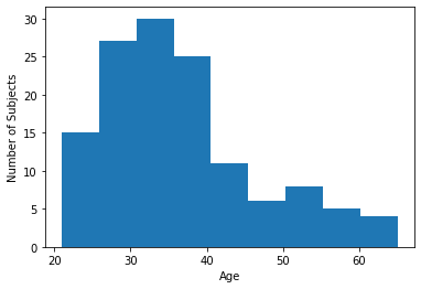
Let’s plot the distribiton of one variable in our data

plt.hist(df['age'], bins=9)
plt.xlabel("Age")
plt.ylabel("Number of Subjects")

Text(0, 0.5, 'Number of Subjects')

_images/module-01-02_Working-with-Data_62_1.png

Let’s see what percentage of subjects have a below-average score:

mean_age = np.mean(df['age'])
frac_below_mean = (df['age'] < mean_age).mean()
print(f"{frac_below_mean:2.1%} of subjects are below the mean")

63.4% of subjects are below the mean

We can also see this by adding the average score to the histogram plot:

plt.hist(df['age'], bins=9)
plt.xlabel("Age")
plt.ylabel("Number of Subjects")

plt.axvline(mean_age, color="orange", label="Mean Age")
plt.legend();
plt.show();

_images/module-01-02_Working-with-Data_66_0.png

Comparing mean and median

med_age = np.median(df['age'])

plt.hist(df['age'], bins=9)
plt.xlabel("Age")
plt.ylabel("Number of Subjects")

plt.axvline(mean_age, color="orange", label="Mean Age")
plt.axvline(med_age, color="black", label="Median Age")

plt.legend();
plt.show();

_images/module-01-02_Working-with-Data_68_0.png

Working with Data

Contents