Nonlinear Modeling
Contents
![]()
Nonlinear Modeling
This tutorial was inspired by and adapted from the Neuromatch Academy tutorials [CC BY 4.0], using a nonlinear hyperbolic model to assess social discounting.
Goals of this tutorial
from scipy.optimize import minimize
from scipy import stats
import numpy as np, pandas as pd
import requests
import matplotlib.pyplot as plt
%matplotlib inline
What is a nonlinear model?
Recall the general linear model, in which the multivariate relationship between a dependent variable (\(y\)) can be expressed as a linear combination of independent variables (\(x_d\)) that are multiplied by a weighted parameter or slope (\(\beta_d\)), plus some noise (\(\epsilon\)):
where \(\beta_0\) is the intercept and \(d\) is the number of features (it is also the dimensionality of our input).
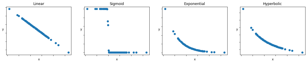
Nonlinear modeling simply implies that the relationship between \(y\) and \(x_d\) is more than a linear combination. Some common examples of nonlinear models include
Sigmoid function:
\(y=\frac{1}{1 + exp(\beta_0 + \beta_1x_1)}\)
Exponential function:
\(y = \beta_0*exp(-\beta_1x_1)\)
Hyperbolic function:
\(y=\frac{\beta_0}{1 + \beta_1x_1}\)
# Let's plot some of these examples:
np.random.seed(2021)

b0 = 1
b1 = .04
b2 = 1.5
b3 = .0125
b4 = 2.67

x1 = np.random.normal(10, 20,
                      size=(100,1))

noise = np.random.randn(100).reshape((100,1))

y = {'Linear': (b0 - b1*x1).reshape((100,1)),
     'Sigmoid': ( ( 1 / (1 + np.exp(b2 + b4*x1)) )).reshape((100,1)),
     'Exponential': (80*np.exp(-b1*x1)).reshape((100,1)),
     'Hyperbolic': ((80/(1 + b3*x1))).reshape((100,1))}
fig, axes = plt.subplots(ncols=4, figsize=(18, 3))

for (key, values), ax in zip(y.items(), axes):

    # True data
    ax.scatter(x1, values)  # our data scatter plot

    ax.set(title= fr'{key}')

    ax.set_xticklabels('')
    ax.set_yticklabels('')
    ax.set_xlabel('x')
    ax.set_ylabel('y', rotation=0)

plt.show()
A case for nonlinear modeling: Social Discounting
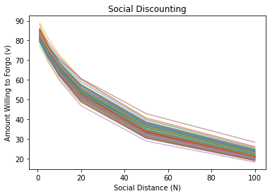
Now that we have a better understanding about some nonlinear models, let’s see how we can apply them to understand people’s prosocial preferences towards close others versus distant strangers. We will fit different models to understand the phenomenon known as social discounting, which describes how the amount of resources that individuals are willing to sacrifice for others (\(v\)) decreases as a hyperbolic function of social distance (\(N\)) (Jones & Rachlin, 2006).
First, let’s simulate some data to get a better intuition about the parameters in the models (the intercept \(v_0\) and slope \(k\)):
np.random.seed(2021)

v0 = np.random.normal(85, 2,
                      size=(100,))

k = np.random.normal(.03, .005,
                      size=(100,))

N = np.array([1,2,5,10,20,50,100])

v = []
for i in range(100):
    v.append((v0[i] / (1 + k[i]*N)) + noise[i])
    plt.plot(N, v[i], alpha=.5)

plt.title('Social Discounting')
plt.ylabel('Amount Willing to Forgo (v)')
plt.xlabel('Social Distance (N)')
plt.show()
Model Parameters
We have two “free” parameters in our hyperbolic model: the intercept (\(v0\)) and slope (\(k\)). The intercept (\(v0\)) represents the value of “amount willing to forgo” (\(v\)) when social distance (\(N\)) equals \(0\). In other words, this is how much an individual values outcomes for him/herself (the undiscounted value of the outcomes)—a larger \(v0\) would indicate that individuals value outcomes for themselves more (note that this parameter is somewhat difficult to interpret, so it is a common practice to add \(+ 1\) to social distance so that the intercept represents the amount willing to forgo for \(N=1\)). The slope (\(k\)) measures the degree of discounting—a smaller \(k\) describes more prosocial (or less selfish) choices for distant others while a larger \(k\) describes more selfish (or less prosocial) choices for distant others.
To start off, let’s create three functions in Python that compute \(v\) (amount willing to forgo) as a function of \(N\) (social distance).
In both the exponential and hyperbolic case, we want to estimate the intercepts (\(v_0\)) and discounting rates (\(k\)) for each participant. We can compute these by minimizing the mean squared error (just like last time).
def mse_linear(params, N, v):

    v0, k = params
    v_fit = v0 + k*N

    mse = np.mean((v - v_fit)**2)

    return mse
def mse_exponential(params, N, v):

    v0, k = params
    v_fit = v0*np.exp(-k*N)

    mse = np.mean((v - v_fit)**2)

    return mse
def mse_hyperbolic(params, N, v):

    v0, k = params
    v_fit = (v0 / (1 + k*N))

    mse = np.mean((v - v_fit)**2)

    return mse
# initialize dictionary to store results
results = {"lin": [],
           "exp": [],
           "hyp": []}

# minimize MSE for linear function using scipy.optimize.minimize
results["lin"] = minimize(mse_linear, # objective function
                          (85, -.3), # estimated starting points
                          args=(N, v), # arguments
                          bounds=((50,100),(-1,1)),
                          tol=1e-3)

# minimize MSE for hyperbolic function using scipy.optimize.minimize
results["exp"] = minimize(mse_exponential, # objective function
                          (92, .6), # estimated starting points
                          args=(N, v), # arguments
                          bounds=((50,100),(0,1)),
                          tol=1e-3)

# minimize MSE for hyperbolic function using scipy.optimize.minimize
results["hyp"] = minimize(mse_hyperbolic, # objective function
                          (70, .05), # estimated starting points
                          args=(N, v), # arguments
                          bounds=((50,100),(0,1)),
                          tol=1e-3)

print(f'Linear: v0 = {results["lin"].x[0]:.2f}, k = {results["lin"].x[1]:.3f}, MSE = {results["lin"].fun:.2f}')
print(f'Exponential: v0 = {results["exp"].x[0]:.2f}, k = {results["exp"].x[1]:.3f}, MSE = {results["exp"].fun:.2f}')
print(f'Hyperbolic: v0 = {results["hyp"].x[0]:.2f}, k = {results["hyp"].x[1]:.3f}, MSE = {results["hyp"].fun:.2f}')
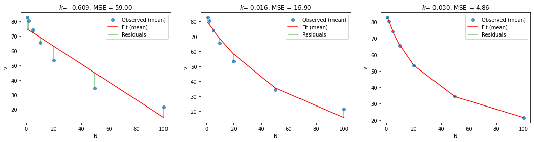
Linear: v0 = 75.27, k = -0.609, MSE = 59.00
Exponential: v0 = 80.75, k = 0.016, MSE = 16.90
Hyperbolic: v0 = 85.20, k = 0.030, MSE = 4.86
fig, axes = plt.subplots(ncols=3, figsize=(18, 4))
for (model, fits), ax in zip(results.items(), axes):

    # True data
    v_mean = np.mean(v, axis=0)
    ax.scatter(N, v_mean,
               alpha = .75,
               label = 'Observed (mean)')  # our data scatter plot

    v0, k = fits.x
    mse_val = fits.fun

    # Compute and plot predictions
    if model == "lin":
        v_hat = v0 + k * N
    elif model == "exp":
        v_hat = v0*np.exp(-k*N)
    elif model == "hyp":
        v_hat = v0 / (1 + k*N)

    ax.plot(N, v_hat, color='r', label='Fit (mean)')  # our estimated model

    # plot residuals
    vmin = np.minimum(v_mean, v_hat)
    vmax = np.maximum(v_mean, v_hat)

    ax.vlines(N, vmin, vmax, 'g', alpha=0.5, label='Residuals')

    ax.set(
      title= fr'$k$= {k:.3f}, MSE = {mse_val:.2f}',
      xlabel='N',
      ylabel='v')

axes[0].legend()
axes[1].legend()
axes[2].legend()
plt.show()
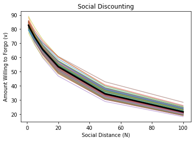
Note that all of these model fits assume a fixed intercept (\(v_o\)) and fixed slope (\(k\)) across participants—in other words, these are the average values across the entire sample.
In reality, we know that intercepts and slopes vary across participants, and can plot the differences below.
# plot all individual subjects
for v_subj in v:
    plt.plot(N, v_subj, alpha=.5)

# plot mean model fit
v_hat = results["hyp"].x[0] / (1 + results["hyp"].x[1]*N)
plt.plot(N, v_hat,
         color='black',
         linewidth=3,
         label='Fit (mean)')  # our estimated model

plt.title('Social Discounting')
plt.ylabel('Amount Willing to Forgo (v)')
plt.xlabel('Social Distance (N)')
plt.show()
# See small differences between fitted and observed values
print(f'{v_hat} -- Fits')
print(f'{v_mean} -- Observed')
[82.74082909 80.42375604 74.19083834 65.7039711  53.47069094 34.30767545
 21.47846287] -- Fits
[82.80278641 80.45272539 74.15481504 65.62721642 53.40723605 34.34937097
 21.58152985] -- Observed
Thus, it might be better to make inferences with our data by allowing the intercepts and slopes to vary across participants. Fitting separate models for each participant is one way (of many) to accomplish this.
# initialize a DataFrame, with columns corresponding to params ['v0', k] and rows corresponding to subjects
res_df = pd.DataFrame(columns=['v0', 'k'])

for subj_id, subj_v in enumerate(v):

    # minimize MSE for hyperbolic function using scipy.optimize.minimize
    fit = minimize(mse_hyperbolic, # objective function
                   (85, .05), # estimated starting points
                   args=(N, subj_v), # arguments
                   bounds=((50,100),(0,1)),
                   tol=1e-3)

    res_df.loc[subj_id, 'v0'] = fit.x[0]
    res_df.loc[subj_id, 'k'] = fit.x[1]
    res_df.loc[subj_id, 'MSE'] = fit.fun

    print(f'subject {subj_id}: v0 = {fit.x[0]:.2f}, k = {fit.x[1]:.3f}, MSE = {fit.fun:.2f}')
subject 0: v0 = 87.34, k = 0.027, MSE = 0.01
subject 1: v0 = 86.74, k = 0.032, MSE = 0.00
subject 2: v0 = 85.18, k = 0.035, MSE = 0.04
subject 3: v0 = 83.00, k = 0.028, MSE = 0.00
subject 4: v0 = 86.56, k = 0.032, MSE = 0.01
subject 5: v0 = 84.06, k = 0.032, MSE = 0.01
subject 6: v0 = 86.89, k = 0.028, MSE = 0.00
subject 7: v0 = 86.93, k = 0.033, MSE = 0.01
subject 8: v0 = 85.61, k = 0.032, MSE = 0.01
subject 9: v0 = 85.08, k = 0.026, MSE = 0.01
subject 10: v0 = 84.65, k = 0.027, MSE = 0.01
subject 11: v0 = 83.70, k = 0.032, MSE = 0.00
subject 12: v0 = 85.19, k = 0.027, MSE = 0.01
subject 13: v0 = 83.93, k = 0.024, MSE = 0.03
subject 14: v0 = 82.90, k = 0.038, MSE = 0.14
subject 15: v0 = 87.24, k = 0.030, MSE = 0.00
subject 16: v0 = 82.73, k = 0.033, MSE = 0.01
subject 17: v0 = 83.61, k = 0.025, MSE = 0.02
subject 18: v0 = 82.53, k = 0.031, MSE = 0.00
subject 19: v0 = 85.92, k = 0.031, MSE = 0.00
subject 20: v0 = 83.91, k = 0.032, MSE = 0.00
subject 21: v0 = 91.07, k = 0.035, MSE = 0.04
subject 22: v0 = 88.52, k = 0.034, MSE = 0.03
subject 23: v0 = 85.38, k = 0.031, MSE = 0.00
subject 24: v0 = 85.26, k = 0.034, MSE = 0.02
subject 25: v0 = 85.56, k = 0.031, MSE = 0.00
subject 26: v0 = 88.74, k = 0.037, MSE = 0.09
subject 27: v0 = 86.92, k = 0.026, MSE = 0.01
subject 28: v0 = 83.56, k = 0.028, MSE = 0.01
subject 29: v0 = 86.26, k = 0.031, MSE = 0.00
subject 30: v0 = 88.35, k = 0.032, MSE = 0.01
subject 31: v0 = 87.59, k = 0.028, MSE = 0.00
subject 32: v0 = 87.90, k = 0.037, MSE = 0.09
subject 33: v0 = 84.37, k = 0.031, MSE = 0.00
subject 34: v0 = 85.88, k = 0.032, MSE = 0.00
subject 35: v0 = 85.53, k = 0.032, MSE = 0.01
subject 36: v0 = 83.40, k = 0.032, MSE = 0.01
subject 37: v0 = 86.35, k = 0.037, MSE = 0.11
subject 38: v0 = 79.91, k = 0.032, MSE = 0.01
subject 39: v0 = 85.62, k = 0.029, MSE = 0.00
subject 40: v0 = 85.60, k = 0.031, MSE = 0.00
subject 41: v0 = 86.42, k = 0.032, MSE = 0.01
subject 42: v0 = 84.90, k = 0.027, MSE = 0.01
subject 43: v0 = 87.15, k = 0.032, MSE = 0.00
subject 44: v0 = 81.64, k = 0.027, MSE = 0.01
subject 45: v0 = 87.58, k = 0.031, MSE = 0.00
subject 46: v0 = 82.66, k = 0.024, MSE = 0.02
subject 47: v0 = 88.35, k = 0.037, MSE = 0.11
subject 48: v0 = 83.87, k = 0.034, MSE = 0.03
subject 49: v0 = 83.54, k = 0.029, MSE = 0.00
subject 50: v0 = 87.04, k = 0.032, MSE = 0.00
subject 51: v0 = 82.67, k = 0.031, MSE = 0.00
subject 52: v0 = 83.27, k = 0.025, MSE = 0.02
subject 53: v0 = 84.08, k = 0.036, MSE = 0.07
subject 54: v0 = 87.91, k = 0.035, MSE = 0.04
subject 55: v0 = 83.63, k = 0.019, MSE = 0.04
subject 56: v0 = 83.40, k = 0.023, MSE = 0.03
subject 57: v0 = 84.98, k = 0.036, MSE = 0.08
subject 58: v0 = 88.32, k = 0.034, MSE = 0.03
subject 59: v0 = 82.08, k = 0.025, MSE = 0.02
subject 60: v0 = 86.55, k = 0.024, MSE = 0.03
subject 61: v0 = 85.16, k = 0.032, MSE = 0.01
subject 62: v0 = 85.18, k = 0.024, MSE = 0.02
subject 63: v0 = 86.37, k = 0.030, MSE = 0.00
subject 64: v0 = 85.07, k = 0.029, MSE = 0.00
subject 65: v0 = 84.85, k = 0.035, MSE = 0.06
subject 66: v0 = 84.30, k = 0.033, MSE = 0.01
subject 67: v0 = 88.06, k = 0.036, MSE = 0.08
subject 68: v0 = 87.70, k = 0.033, MSE = 0.02
subject 69: v0 = 84.96, k = 0.033, MSE = 0.02
subject 70: v0 = 86.41, k = 0.026, MSE = 0.01
subject 71: v0 = 85.45, k = 0.024, MSE = 0.02
subject 72: v0 = 81.49, k = 0.030, MSE = 0.00
subject 73: v0 = 83.34, k = 0.030, MSE = 0.00
subject 74: v0 = 82.40, k = 0.031, MSE = 0.00
subject 75: v0 = 83.74, k = 0.032, MSE = 0.00
subject 76: v0 = 86.06, k = 0.027, MSE = 0.01
subject 77: v0 = 88.30, k = 0.029, MSE = 0.00
subject 78: v0 = 85.50, k = 0.033, MSE = 0.02
subject 79: v0 = 84.61, k = 0.024, MSE = 0.02
subject 80: v0 = 85.92, k = 0.033, MSE = 0.01
subject 81: v0 = 84.83, k = 0.030, MSE = 0.00
subject 82: v0 = 83.61, k = 0.028, MSE = 0.00
subject 83: v0 = 87.29, k = 0.032, MSE = 0.01
subject 84: v0 = 84.32, k = 0.024, MSE = 0.02
subject 85: v0 = 88.26, k = 0.033, MSE = 0.02
subject 86: v0 = 86.83, k = 0.033, MSE = 0.01
subject 87: v0 = 84.54, k = 0.024, MSE = 0.02
subject 88: v0 = 91.47, k = 0.026, MSE = 0.01
subject 89: v0 = 81.25, k = 0.023, MSE = 0.03
subject 90: v0 = 81.40, k = 0.025, MSE = 0.02
subject 91: v0 = 87.81, k = 0.031, MSE = 0.00
subject 92: v0 = 82.99, k = 0.027, MSE = 0.01
subject 93: v0 = 88.16, k = 0.023, MSE = 0.03
subject 94: v0 = 81.63, k = 0.023, MSE = 0.03
subject 95: v0 = 83.84, k = 0.026, MSE = 0.02
subject 96: v0 = 84.69, k = 0.033, MSE = 0.01
subject 97: v0 = 85.31, k = 0.027, MSE = 0.01
subject 98: v0 = 85.96, k = 0.027, MSE = 0.01
subject 99: v0 = 82.42, k = 0.027, MSE = 0.01
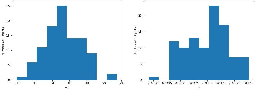
We can plot the distributions of \(v_0\) and \(k\) across participants
fig, axes = plt.subplots(ncols=2, figsize=(15,5))

axes[0].hist(res_df['v0'], bins=10)
axes[0].set(ylabel="Number of Subjects", xlabel="v0")

axes[1].hist(res_df['k'], bins=10)
axes[1].set(ylabel="Number of Subjects", xlabel="k")

plt.show()
Model comparison
Above, we can see that the hyperbolic model fits the data best, but typically the best fitting model isn’t so obvious. Thus, we can use methods such as \(R^2\) or the Bayesian Information Criterion (\(BIC\)) to compare model fits. The model with the lowest \(BIC\) value is the best fitting model in a finite set of models.
The \(BIC\) penalizes free parameters (see constant term: \(k*ln(n)\)):
Here, \(n\) is the total number of observations in your sample (e.g., sample size), \(p\) the number of parameters estimated by the model (we are estimating two parameters in our model: \(v0\) and \(k\)), and \(MSE\) is the mean sqauared error of the model. Remember that a lower \(BIC\) value is better; Adding the term \(p*ln(n)\) penalizes the model fit by the number of free parameters.
def calculate_bic(sample_size, mse, num_params):
    bic = -2 * np.log(mse) + num_params * np.log(sample_size)
    return bic
# calculate the Bayesian Information Criterion (bic)
for key, output in results.items():
    bic = calculate_bic(len(v_mean), output.fun, 2)
    print(f'{key} (BIC): {bic:.3f}')
lin (BIC): -4.263
exp (BIC): -1.763
hyp (BIC): 0.730
We can now show that the hyperbolic model is the model with the lowest \(BIC\) value (out of the models tested above).
Fitting actual data to models
Now that we’ve seen two examples of simulating data and model parameter recovery. Let’s try to fit actual data to these models.
We will use a subset of the data from Vekaria et al. (2017).
# First let's load in the data

# here, we are just going to download data from the web (no need to edit these lines, but try to figure out what they are doing)
url = 'https://raw.githubusercontent.com/shawnrhoads/gu-psyc-347/master/docs/static/data/Vekaria-et-al-2017_data.csv'
df = pd.read_csv(url, index_col='subject')
print(df.head())
          1   2   5  10  20  50  100
subject
102      85  85  85  85  85  65   85
106      85  85  -5   5   5   5    5
107      85  85  85  85  85   5    5
113      85  55  65  55  25  15    5
114      65  55  45  55  45  15   15
We can see that our data are formatted with participants as rows and amounts willing to forgo at each social distance as columns. To use our functions above, we will need to make sure our \(v\) data have shape (n_subjects, 7).
Let’s convert the pd.DataFrame to a np.array:
vekaria_data = df.values

print(vekaria_data.shape)
(25, 7)
First, let’s fit all of the data together, with fixed intercepts and slopes, for both the hyperbolic model and the exponential model.
fit1 = minimize(mse_hyperbolic, # objective function
               (85, .05), # estimated starting points
               args=(N, df.iloc[:,0:7].values), # arguments
               bounds=((0,80),(0,1)),
               tol=1e-3)

# minimize MSE for exponential function using scipy.optimize.minimize
fit2 = minimize(mse_exponential, # objective function
               (85, .05), # estimated starting points
               args=(N, df.iloc[:,0:7].values), # arguments
               bounds=((0,80),(0,1)),
               tol=1e-3)
# fig, axes = plt.subplots()
fig = plt.figure()

plt.scatter(N, np.mean(df.iloc[:,0:7].values, axis=0), label='Observed (mean)')
plt.plot(N, fit1.x[0] / (1 + fit1.x[1]*N), label='Hyperbolic')
plt.plot(N, fit2.x[0] * np.exp(-fit1.x[1]*N), label='Exponential')
plt.legend()

plt.show()
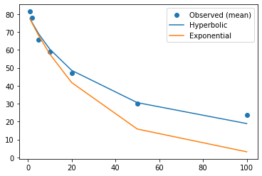
Based on this plot, we can clearly see how much better the hyperbolic model is at explaining the variance in the data. We can confirm this again using the \(BIC\).
# calculate the Bayesian Information Criterion (bic)
for label, output in zip(['hyperbolic', 'exponential'], [fit1, fit2]):
    bic = calculate_bic(len(vekaria_data), output.fun, 2)
    print(f'{label} (BIC): {bic:.3f}')
hyperbolic (BIC): -6.567
exponential (BIC): -6.668
# initialize a DataFrame, with columns corresponding to params ['v0', k] and rows corresponding to subjects
res_vekaria = pd.DataFrame(columns=['v0', 'k'])

for subj_id, subj_v in zip(df.index, vekaria_data):

    # minimize MSE for hyperbolic function using scipy.optimize.minimize
    fit = minimize(mse_hyperbolic, # objective function
                   (85, .05), # estimated starting points
                   args=(N, subj_v), # arguments
                   bounds=((0,80),(0,1)),
                   tol=1e-3)

    res_vekaria.loc[subj_id, 'v0'] = fit.x[0]
    res_vekaria.loc[subj_id, 'k'] = fit.x[1]
    res_vekaria.loc[subj_id, 'MSE'] = fit.fun

    print(f'subject {subj_id}: v0 = {fit.x[0]:.2f}, k = {fit.x[1]:.3f}, MSE = {fit.fun:.2f}')
subject 102: v0 = 80.00, k = 0.000, MSE = 53.53
subject 106: v0 = 80.00, k = 0.301, MSE = 488.09
subject 107: v0 = 80.00, k = 0.024, MSE = 430.10
subject 113: v0 = 79.88, k = 0.074, MSE = 75.61
subject 114: v0 = 62.64, k = 0.033, MSE = 42.86
subject 116: v0 = 80.00, k = 0.000, MSE = 25.00
subject 119: v0 = 80.00, k = 0.021, MSE = 370.64
subject 120: v0 = 79.94, k = 0.087, MSE = 224.61
subject 121: v0 = 80.00, k = 0.000, MSE = 25.00
subject 122: v0 = 80.00, k = 0.003, MSE = 62.99
subject 123: v0 = 79.62, k = 0.110, MSE = 358.13
subject 124: v0 = 79.97, k = 0.062, MSE = 55.33
subject 125: v0 = 80.00, k = 0.019, MSE = 294.43
subject 126: v0 = 80.00, k = 0.006, MSE = 820.72
subject 127: v0 = 80.00, k = 0.030, MSE = 138.29
subject 128: v0 = 80.00, k = 0.000, MSE = 25.00
subject 132: v0 = 80.00, k = 0.024, MSE = 196.97
subject 135: v0 = 80.00, k = 0.056, MSE = 503.05
subject 136: v0 = 79.98, k = 0.089, MSE = 271.09
subject 137: v0 = 80.00, k = 0.021, MSE = 351.20
subject 138: v0 = 80.00, k = 0.024, MSE = 149.32
subject 139: v0 = 80.00, k = 0.220, MSE = 273.89
subject 141: v0 = 79.93, k = 0.083, MSE = 135.05
subject 143: v0 = 56.54, k = 0.036, MSE = 16.84
subject 147: v0 = 80.00, k = 0.361, MSE = 178.55
We can see that some participants did not do very well with model fitting. For most, this is because their “amounts willing to forgo” do not vary across social distances.
To account for this, let’s check which subjects these are.
for subj_id, subj_v in zip(df.index, vekaria_data):
    if all(x==subj_v[0] for x in subj_v):
        print(f'no variation for subject #{subj_id}, {subj_v}')
no variation for subject #116, [85 85 85 85 85 85 85]
no variation for subject #121, [85 85 85 85 85 85 85]
no variation for subject #128, [85 85 85 85 85 85 85]
Three participants sacrificed all of their resources for all social others. Let’s assign k=0 and v0=85 to these participants since there is no variation in their preferences. This is eqivalent to a straight horizontal line (no discounting) at \(v=85\).
# initialize a DataFrame, with columns corresponding to params ['v0', k] and rows corresponding to subjects
hyp_vekaria = pd.DataFrame(columns=['v0', 'k'])

for subj_id, subj_v in zip(df.index, vekaria_data):

    if all(x==subj_v[0] for x in subj_v):
        if np.sum(subj_v)>=595:

            hyp_vekaria.loc[subj_id, 'v0'] = 80 #
            hyp_vekaria.loc[subj_id, 'k'] = 0
            hyp_vekaria.loc[subj_id, 'MSE'] = np.nan

            print(f'assigning k=0 for subject #{subj_id}, {subj_v}')
    else:

        # minimize MSE for hyperbolic function using scipy.optimize.minimize
        fit = minimize(mse_hyperbolic, # objective function
                       (85, .05), # estimated starting points
                       args=(N, subj_v), # arguments
                       bounds=((0,80),(0,1)),
                       tol=1e-3)

        hyp_vekaria.loc[subj_id, 'v0'] = fit.x[0]
        hyp_vekaria.loc[subj_id, 'k'] = fit.x[1]
        hyp_vekaria.loc[subj_id, 'MSE'] = fit.fun

res_vekaria = pd.concat([df, hyp_vekaria], axis=1)
assigning k=0 for subject #116, [85 85 85 85 85 85 85]
assigning k=0 for subject #121, [85 85 85 85 85 85 85]
assigning k=0 for subject #128, [85 85 85 85 85 85 85]
fig, axes = plt.subplots(ncols=2, figsize=(15,5), sharey=True)

axes[0].hist(res_vekaria['v0'], bins=20)
axes[0].set(ylabel="Number of Subjects", xlabel="v0")

axes[1].hist(res_vekaria['k'], bins=20)
axes[1].set(ylabel="Number of Subjects", xlabel="k")

plt.show()
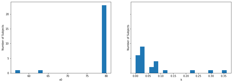
Yay! Now, we can use these data for subsequent analyses! Note the little variation in \(v_0\). Also note that \(k\) is not parametric (e.g., not normally distributed), so we would need to conduct subsequent analyses using non-parametric approaches.