Two-Armed Bandit
Contents
![]()
Two-Armed Bandit
This tutorial was inspired by and adapted from Models of Learning and the Neuromatch Academy tutorials [CC BY 4.0].
In this tutorial, we will complete a learning task where your goal will be to maximize the amount of points you can earn by sampling the reward distribution from one of two slot machines. This is also known as a two-armed bandit task.
Getting started
To start off, we will (0) open Terminal (Mac/Linux) or Anaconda Prompt (Windows). We will then (1) activate our course environment, (2) change the directory to gu-psyc-347-master (or whatever you named your course directory that we downloaded at the beginning of the semester; you can also download it here), (3) update the directory contents using git, and finally (4) check that our course environment is up-to-date.
Items 1-4 can be accomplished using the following four commands in the Terminal / Prompt:
conda activate gu-psyc-347
cd gu-psyc-347-master
git pull origin master
conda env update --file course-env.yml
Running the task
The task we will run was built using PsychoPy, which is a “free cross-platform package allowing you to run a wide range of experiments in the behavioral sciences (neuroscience, psychology, psychophysics, linguistics).” PsychoPy is a great tool to use to create and run behavioral experiments because it is open-source and is backed by a huge community of developers and users!
To run the course, check that you now have a directory called two-armed-bandit in your course directory. If your course directory is called gu-psyc-347, the directory structure should look something like this:
gu-psyc-347
├── course-env.yml
├── LICENSE
├── README.md
├── requirements.txt
├── docs
│    ├── static
│    ├── solutions
│    ├── tasks
│          └── two-armed-bandit
│                    ├── two-armed-bandit.psyexp
│                    ├── two-armed-bandit.py
│                    ├── two-armed-bandit_lastrun.py
│                    ├── data
│                    ├── orders
│                    ├── stimuli
Once you are able to confirm that your directory looks like this, then we can start the experiment!
Before you run the experiment, your instructor will give you a number ranging from 0-13. This will be the participant ID number that you input at the beginning of the task. Please keep this number in mind.
You can run the experiment by using this command in Terminal (Mac/Linux) or Anaconda Prompt (Windows): python two-armed-bandit.py
The task will take roughly 8 minutes to complete.
Task Debrief
You just completed 72 trials! 2 slot machines were presented on every trial, each associated with a certain probability of reward.
Did you learn which slot machine had the greater payout probability?
You were not told this, but the payout probabilities for the blue and orange machines were coupled. There was always one ‘good’ option and one ‘bad’ option.
In breakout rooms, discuss with a partner the following questions and report back to the group:
What did you like about the task?
What didn’t you like about the task?
What do you think the probablities of the slot machines were? (e.g., 50/50, 25/75, 60/40, 80/20). Do you think you and your partner(s) had the same slot machine reward probabilities? Why or why not?
Why do you think the position of the machines were randomized on each trial? In other words, why wasn’t the orange slot machine always on the same side?
How many trials did it take you to learn which slot machine was better (if at all)? If there were less trials (<72 trials) or more trials (>72 trials), do you think you would be better or worse at learning?
Were there times when you expected to receive a rewarding outcome but didn’t? How did that change your behavior on the next trial?
When you didn’t get the outcome you expected, how often did you switch your choice on the next trial? What parameter in the Rescorla-Wagner model might correspond to this phenomenon? (Recall the equation from class: \( Q^k_{t+1} = Q^k_t + \alpha (r_t - Q^k_t) \))
How “explorative” was your behavior when you were completing the task? In other words, even if you learned which slot machine had the greater payout probability, how often did you sample the other one just to see what would happen? Do you think we can model this as well?
Viewing your behavior
Let’s plot our behavior from the task to see how we did! In order to load your data into this Jupyter Notebook, recall your participant ID. The instructor’s ID was 00, so that is what we will use in the examples. Replace the following id_num='00' with your ID below.
id_num = '00' # this is the only line of code you need to change
We will now load our usual packages into memory, so we can view, manipulate, and plot our behavioral data.
import pandas as pd
import numpy as np
import matplotlib.pyplot as plt
%matplotlib inline
After completing the task, your data was saved to tasks/two-armed-bandit/data/. Let’s load our behavioral data in.
datafile = f'https://raw.githubusercontent.com/shawnrhoads/gu-psyc-347/master/docs/tasks/two-armed-bandit/data/sub-{id_num}_task-two-armed-bandit.csv'
df = pd.read_csv(datafile)
display(df.head())
| subject | type | condition | goal | block | block_num | block_instr_text | trial_num | stim_0 | stim_0_value | ... | outcomeDescr | outcome | feedback_text.started | feedback_text.stopped | participant | date | expName | psychopyVersion | frameRate | Unnamed: 60 | |
|---|---|---|---|---|---|---|---|---|---|---|---|---|---|---|---|---|---|---|---|---|---|
| 0 | 0 | 0 | self | win | self_win | 1 | Play to WIN points | 0 | stimuli/slot1_up.jpg | 1 | ... | self avoid win | 0 | 105.138390 | None | 0 | 2021_Mar_01_2315 | two-armed-bandit | 2021.1.0 | 60.000312 | NaN |
| 1 | 0 | 0 | self | win | self_win | 1 | Play to WIN points | 1 | stimuli/slot1_up.jpg | 1 | ... | self win | 1 | 108.754971 | None | 0 | 2021_Mar_01_2315 | two-armed-bandit | 2021.1.0 | 60.000312 | NaN |
| 2 | 0 | 0 | self | win | self_win | 1 | Play to WIN points | 2 | stimuli/slot1_up.jpg | 1 | ... | self win | 1 | 112.338230 | None | 0 | 2021_Mar_01_2315 | two-armed-bandit | 2021.1.0 | 60.000312 | NaN |
| 3 | 0 | 0 | self | win | self_win | 1 | Play to WIN points | 3 | stimuli/slot1_up.jpg | 1 | ... | self win | 1 | 115.921452 | None | 0 | 2021_Mar_01_2315 | two-armed-bandit | 2021.1.0 | 60.000312 | NaN |
| 4 | 0 | 0 | self | win | self_win | 1 | Play to WIN points | 4 | stimuli/slot1_up.jpg | 0 | ... | self avoid win | 0 | 119.421379 | None | 0 | 2021_Mar_01_2315 | two-armed-bandit | 2021.1.0 | 60.000312 | NaN |
5 rows × 61 columns
Cumulative points over trials
First, let’s plot our culmulative points over trials!
# points over trials
plt.plot(df['trial_num'], df['cumulativePts_self'])
plt.xlabel('trials')
plt.ylabel('cumulative points')
plt.title(f'Total points: {df.cumulativePts_self.values[-1]}')
plt.show()
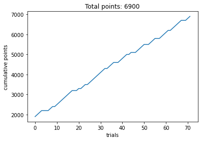
How did you do? When didn’t your points increase? Does this have any relationship with the machine you chose? Let’s overlay point accumulation with behavior.
Choices on each trial
We can also plot the choices we made on each trial. Let’s plot the choices for the slot machine with the highest probability.
# compute which machine yielded rewards more frequently
if df['stim_0_value'].mean() > df['stim_1_value'].mean():
    better_machine = 'stim_0'
    better_machine_val = 'stim_0_value'
    better_machine_choice = 'chosen_stim_0'
else:
    better_machine = 'stim_1'
    better_machine_val = 'stim_1_value'
    better_machine_choice = 'chosen_stim_1'

# plot choices for this machine
plt.plot(df['trial_num'], df[better_machine_choice], '+')
plt.xlabel('trials')
plt.ylabel('choice (1=better choice)')
plt.title(f'Chose better machine {df[better_machine_choice].sum()} times out of {len(df[better_machine_choice])}')
plt.show()
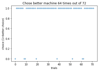
Did you learn that this machine was better? How did your choices correspond with the actual outcome associated with the machine on a given trial? (Remember: the machine yielded rewards with a certain probability)
Actual values of the machine over trials
Let’s plot the actual values associated with the machine over trials. These aren’t the actual outcomes displayed to you during the task.
# plot values for this machine
plt.plot(df['trial_num'], df[better_machine_val], '--')
plt.xlabel('trials')
plt.ylabel('value')
plt.title(f'Values associated with better machine over trials')
plt.show()
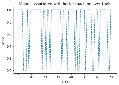
As we can see, the machine was set up to produce varying outcomes over trials (even though this was the better machine). In other words, this machine only yielded rewards with a certain probability.
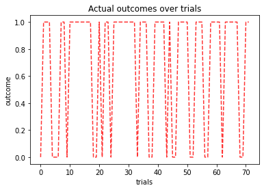
Actual outcomes during the task
We can also plot out the actual outcomes that we observed during the task. These were based on what choices we made on each trial. They might map onto the values over trials fairly well.
plt.plot(df['trial_num'], df['outcome'], 'r--', alpha=.8)
plt.xlabel('trials')
plt.ylabel('outcome')
plt.title(f'Actual outcomes over trials')
plt.show()
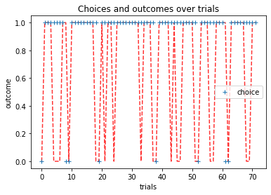
Finally, we can plot both our choices and outcomes over trials. Do our choices reflect the actual outcomes over time?
plt.plot(df['trial_num'], df['outcome'], 'r--', alpha=.8)
plt.plot(df['trial_num'], df[better_machine_choice], '+', label='choice')
plt.xlabel('trials')
plt.ylabel('outcome')
plt.title(f'Choices and outcomes over trials')
plt.legend()
plt.show()
Great! Recall the ten simple rules for computational modeling of behavioral data (Wilson & Collins, 2019). We will be going through these steps throughout this module.
We finished our first step: Experimental Design. At this stage, we can continue to tweak our experiment, or continue onto building models. Before next class, think of a few models we can test using this task. Like we discussed during the lecture, it is unlikely that we are keeping a running average of all of our choices throughout the task. Thus, we might be computing the average in a more “online” way. For example, we could be assigning value and keeping track of this value for each of the slot machines.
We will specify a few models, simulate some data, and then attempt to recover the parameters.